图形学入门笔记3: Path Tracing
Path tracing笔记以及Games101作业7代码相关解读以及实现。笔记包括
- 辐射度量学相关概念
- 渲染方程
- 蒙特卡洛积分
- Path Tracing逻辑。
辐射度量学 (Radiometry)
辐射通量 (Radiant flux (power)) \(\Phi=\frac{\mathrm{d}Q}{\mathrm{d}t}\) Energy per unit time,表示单位时间内光穿过一个截面的光能。
辐射强度 (Radiant intensity),\(I(\omega)=\frac{\mathrm{d}\Phi}{\mathrm{d}\omega}\) Power per unit solid angle,表示单位立体角上的辐射通量。
辐射率 (Radiance),\(L(\mathrm p,\omega)=\frac{\mathrm d^2\Phi(p,\omega)}{\mathrm d \omega\cdot\mathrm dA\cos\theta}\) Power emitted, reflected, transmitted or received by a surface, per unit solid angle, per projected unit area,表示单位立体角,单位投影面积上的辐射通量。这里多出来一个\(\cos \theta\)是因为Lamber's Cosine Law,即阳光在斜照的时候强度会由于倾角变成原来的\(\cos \theta\)倍。
辐照度 (Irradiance),\(E(\mathrm{x})=\frac{\mathrm d\Phi(\mathrm x)}{\mathrm d A}\) Power per unit area incident on a surface point,表示单位面积上的辐射通量。这里有一种记忆方法,在Games104上学到的,将Irradiance拆分成Ir(In)和Radiance记为进入到表面的光照强度。
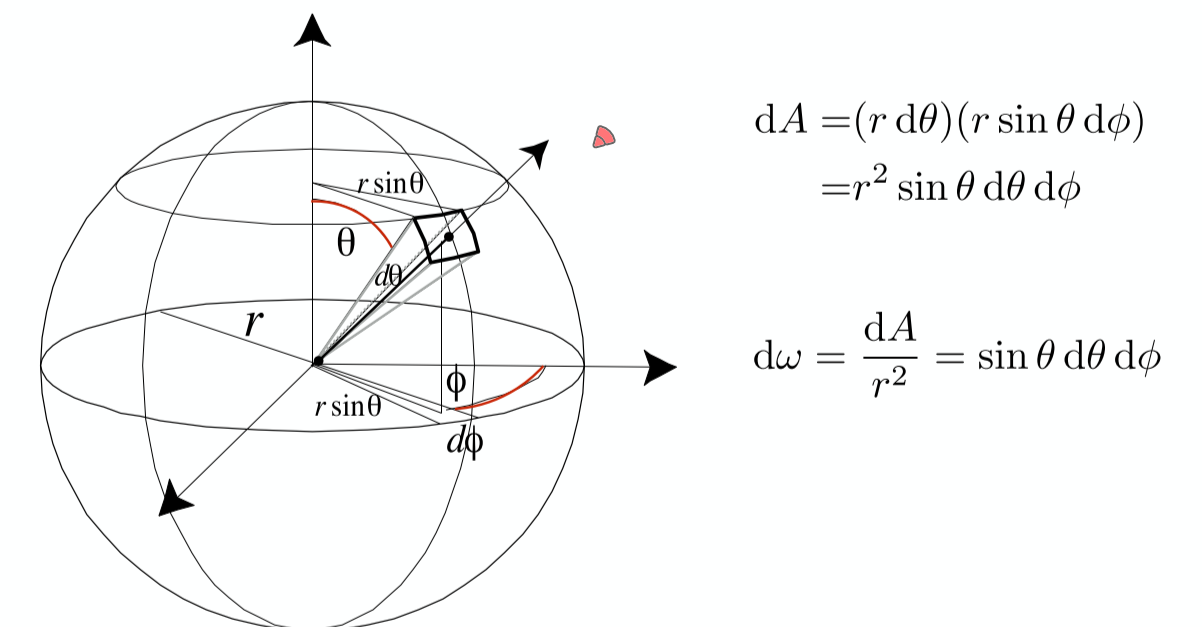
立体角 (Solid Angles)
Bidirectional Reflectance Distribution Function (BRDF)
- 渲染方程 (Rendering Equation) \[ L_o(p,\omega_0)=L_e(p,\omega_0)+\int_{\Omega+}L_i(p,\omega_i)f_r(p,\omega_i,\omega_0)(n\cdot\omega_i)\mathrm d\omega_i \] 其中第一项表示物体本身的发出的光照强度,第二项的积分所包括的内容就是我们的反射函数 (Reflection Function),即 \[ L_r(\mathrm p, \omega_r)=\int_{\Omega+}L_i(p,\omega_i)f_r(p,\omega_i,\omega_0)\cos\theta_i\mathrm d\omega_i \] 其中第一项为入射方向的Radiance,代表从单位立体角方向入射到单位面积上的光照强度,第二项就是双向反射分布函数,他表示以下比值 \[ f_r(\omega_i\rightarrow\omega_r)=\frac{\mathrm dL_r(\omega_r)}{\mathrm dE_i(\omega_i)}=\frac{\mathrm dL_r(\omega_r)}{L_i(\omega_i)\cos\theta_i\mathrm d\omega_i}~~[\frac{1}{\text{sr}}] \] 也就是出射光Radiance与入射光Irradiance的比值,也就是代表了在各个方向上多少光照会被反射出去。这里的积分是对入射光的Radiance进行积分,得到的就是入射光在半球面上的Irradiance,然后和BRDF相乘得到的就是反射出的在单位立体角上的Radiance。
蒙特卡洛积分 (Monte Carlo Integration)
- Monte Carlo estimator \(F_N=\frac{1}{N}\sum^N_{i=1}\frac{f(X_i)}{p(X_i)}\), Example, Basic (Uniform) Monte Carlo estimator \(F_N=\frac{b-a}{N}\sum_{i=1}^Nf(X_i)\)
- Monte Carlo Integration \(\int f(x)\mathrm dx=\frac{1}{N}\sum_{i=1}^N\frac{f(X_i)}{p(X_i)}\) The more samples, the less variance.
路径追踪 (Path Tracing)
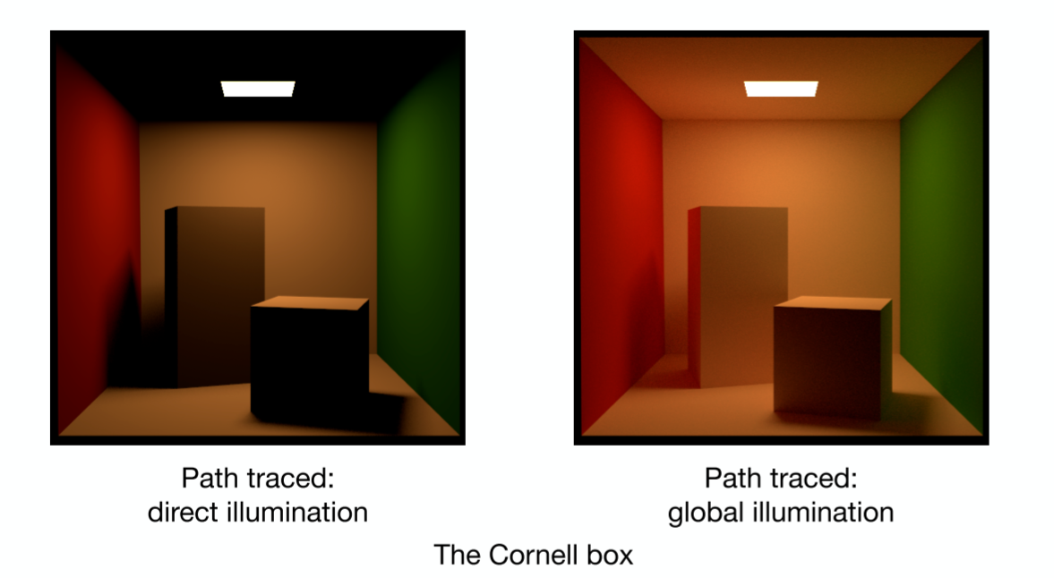
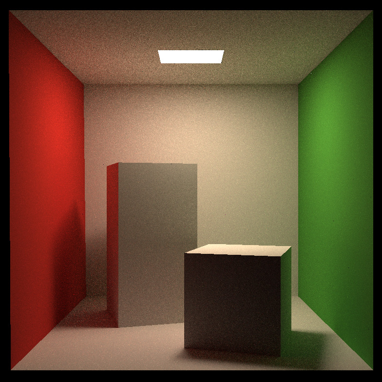
Whitted-style 光线追踪始终采用镜面反射,在光线与diffuse表面相交时停止反射,这一假设会造成一些问题。首先,比如说诸如Glossy (感觉类似磨砂)的效果就无法表现出来。其次,由于不在diffuse表面进行反射,物体之间由于光线反射形成的现象比如说康奈尔Box中的墙面会映射出左右两面墙的红绿两种颜色(如下图)就无法表现出来。
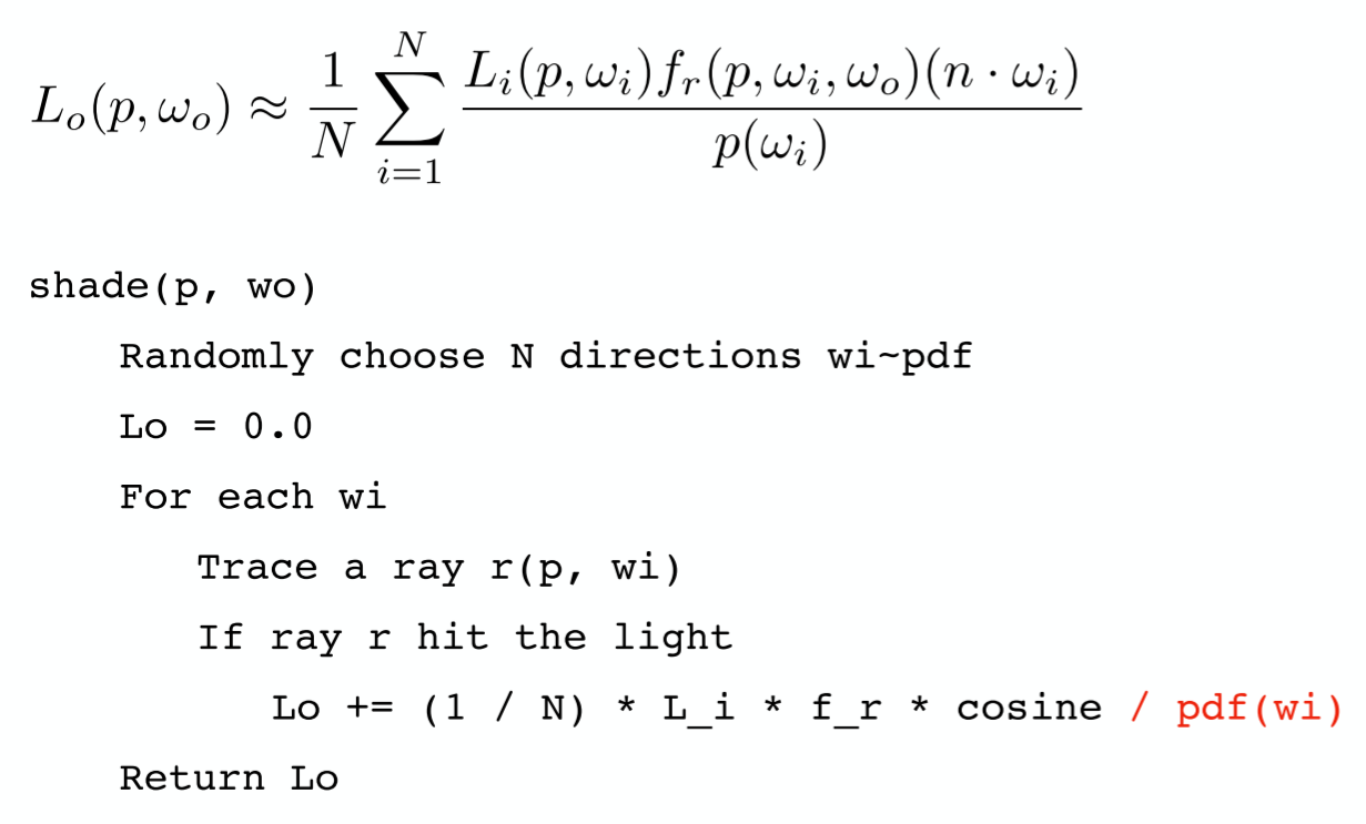
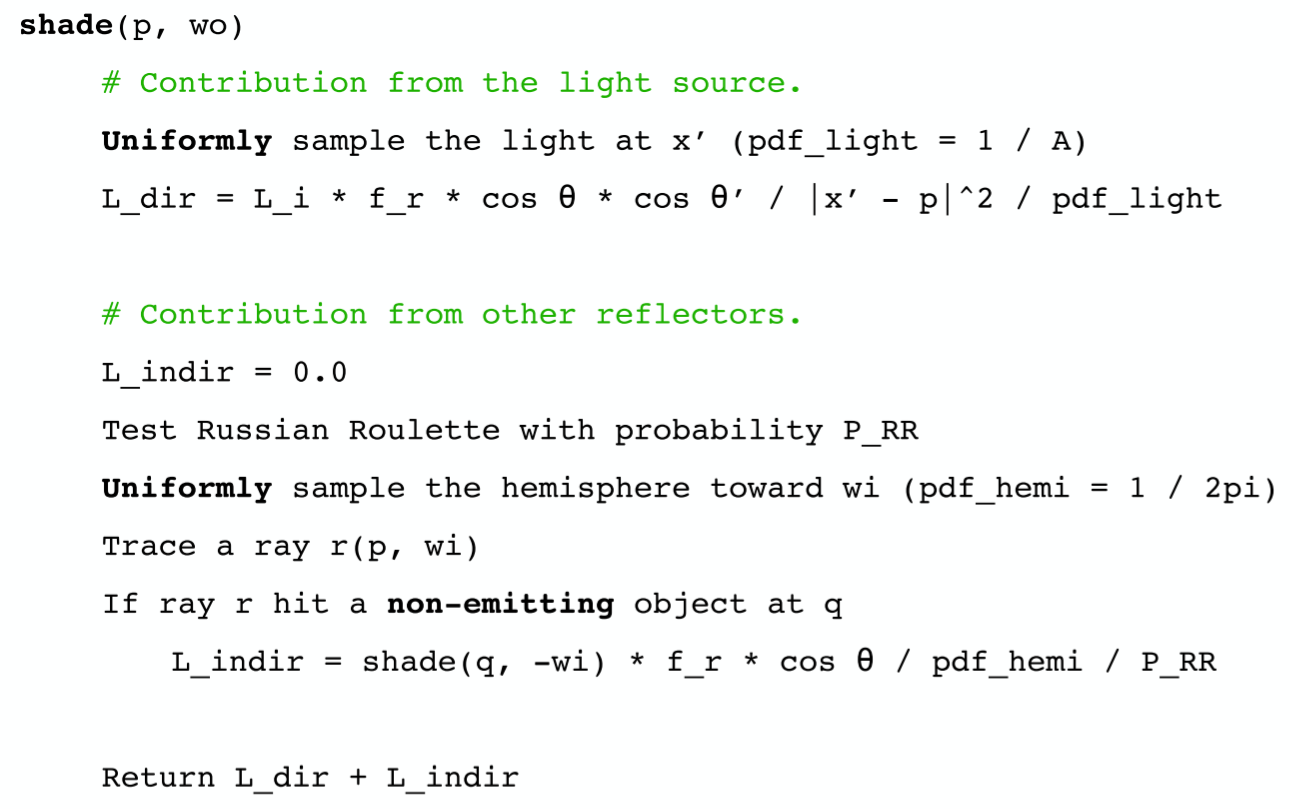
Path tracing使用Rendering Equation进行光照的计算。在计算Rendering Equation中的积分部分时,我们就可以使用Monte Carlo Integration计算。一个简单的Monte Carlo的方法如下图所示 (Direct Illumination),其中的pdf最直观的办法我们可以视为uniform的,也就是\(\mathrm{pdf}=\frac{1}{2\pi}\)。
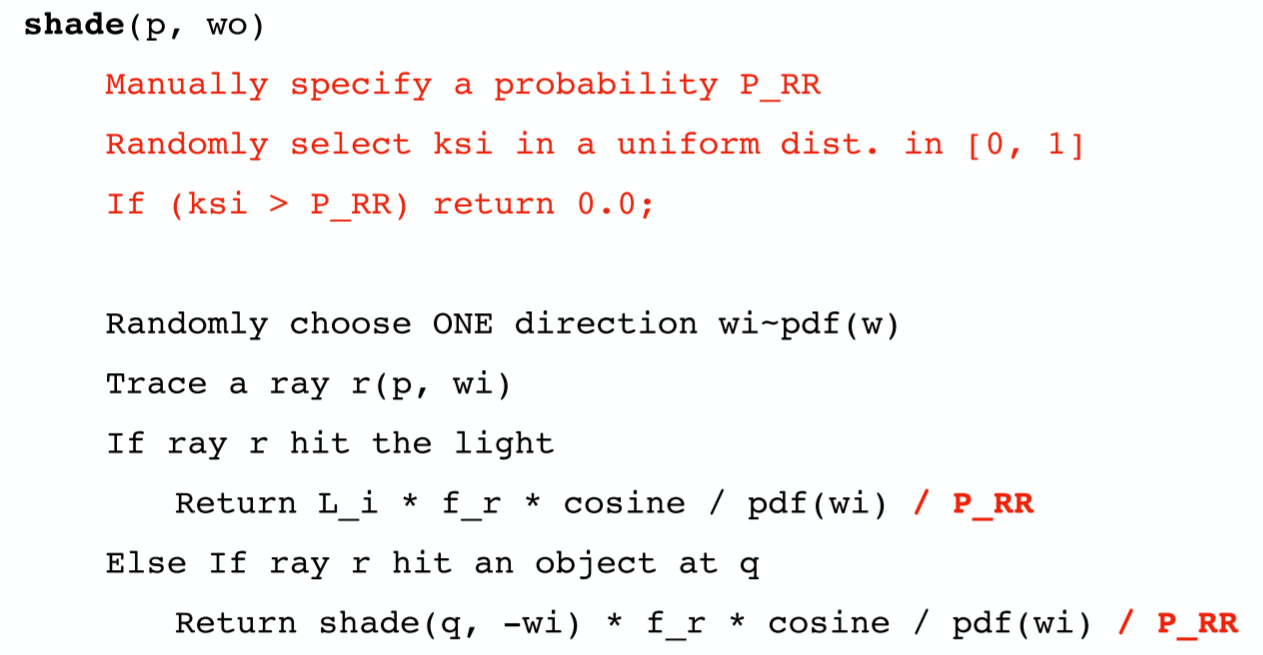
以上是最简单的直接光照的蒙特卡洛积分,然后我们再加上递归的间接光照以及控制递归深度就完成了最终的Path Tracing。为了控制深度,我们使用一种叫做俄罗斯轮盘赌 (Russian Roulette)的方法。非常简单,这种方法就是在每次光线进行反射的时候进行一次随机选择,p的概率继续递归,(1-p)的概率停止,如果继续反射,则我们计算反射的光照强度为\(\frac{L_r(p,\omega_r)}{p}\),这样我们最后根据数学期望得到的光照强度仍然是\(L_r(p,\omega_r)\)。使用后RR的Path Tracing伪代码如下所示。
最后还有一个问题需要解决,使用以上方法进行采样的效率实际上是不高的,因为很多光线实际上是反射不到光源上的,那样就会造成很多浪费。因此,我们可以使用另外一种采样方式,Sampling
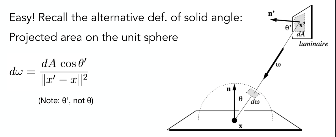
the
Light,从光源处采样。为了实现光源采样,我们可以重写反射方程,将对入射角度\(\omega\)的积分转化为对光源面积\(A\)的积分,由于\(\mathrm d\omega=\frac{\mathrm
dA\cos\theta'}{\Vert x'-x\Vert^2}\)
(由立体角的定义得出),因此 \[
\begin{align}
L_r(\mathrm
p,\omega_r)&=\int_{\Omega+}L_i(x,\omega_i)f_r(x,\omega_i,\omega_0)\cos\theta_i\mathrm
d\omega_i \\
&=\int_{A}L_i(x,\omega_i)f_r(p,\omega_i,\omega_0)\frac{\cos\theta_i\cos\theta'_i}{\Vert
x'-x\Vert^2}\mathrm d\omega_i
\end{align}
\] 
最终版的Path Tracing伪代码如下
作业7
首先,我们需要将上一次作业的几个函数的实现复制粘贴到这里来,包括Triangle::getIntersection()
in
Triangle.hpp,IntersectP(const Ray& ray, const Vector3f& invDir, const std::array<int, 3>& dirIsNeg)
in
Bounds3.hpp以及getIntersection(BVHBuildNode* node, const Ray ray)
in BVH.cpp。代码如下所示
1 | // Triangle.hpp |
完成后确保编译运行都没有问题后,我们再正式开始这次作业的实现,我们只需要对castRay(const Ray ray, int depth)
in Scene.cpp进行实现,代码如下所示
1 | Vector3f Scene::castRay(const Ray &ray, int depth) const |
最终生成的图片,这里为了效果好一点我跑了128的SPP,大概需要跑几个小时,如下图
多线程部分
多线程部分只需要把render()函数中部分渲染相关代码修改为以下内容,对多行像素进行同时渲染。C++多线程教程可以参考C++11
多线程(std::thread)详解_std::thread
查线程名称_sjc_0910的博客-CSDN博客。使用多线程的速度可以看到显著提升
1
2
3
4
5
6
7
8
9
10
11
12
13
14
15
16
17
18
19
20
21
22
23
24
25
26
27
28
29
30
31
32
33
34
35
int spp = 64;
std::cout << "SPP: " << spp << "\n";
const int thread_num = 16;
std::thread th[thread_num];
std::atomic_int process = 0;
int times = scene.height / thread_num;
auto func = [&](uint32_t y_min, uint32_t y_max) {
for (uint32_t j = y_min; j < y_max; ++j) {
int m = j * scene.width;
for (uint32_t i = 0; i < scene.width; ++i) {
// generate primary ray direction
auto x = static_cast<float>((2 * (i + 0.5) / (double) scene.width - 1) * imageAspectRatio * scale);
auto y = static_cast<float>((1 - 2 * (j + 0.5) / (double) scene.height) * scale);
Vector3f dir = normalize(Vector3f(-x, y, 1));
for (int k = 0; k < spp; k++) {
framebuffer[m] += scene.castRay(Ray(eye_pos, dir), 0) / spp;
}
m++;
}
mtx.lock();
process++;
UpdateProgress((float) process / (float) scene.height);
mtx.unlock();
}
};
for (uint32_t i = 0; i < thread_num; ++i) {
th[i] = std::thread(func, i * times, (i + 1) * times);
}
for (int i = 0; i < thread_num; ++i) {
th[i].join();
std::cout << "Join thread " << i << std::endl;
}
UpdateProgress(1.f);
微表面模型
另外,除了多线程还有一个提高部分是微表面模型,这个模型应该只需要去改一下Material相关的部分,只不过这部分目前还是有点不太熟悉,打算等到Games202之后才回过头来做完。
参考资料
GAMES101:作业7_南酒猫的博客-CSDN博客_games101作业7 C++11 多线程(std::thread)详解_std::thread 查线程名称_sjc_0910的博客-CSDN博客